Introduction
Understanding how infectious diseases propagate is a key challenge for the 21st century. Mathematical modelling is a powerful method for studying complex systems that is commonly used in many scientific disciplines. It is widely used to carry out researches on modelling infectious diseases in order to study the mechanisms of transmission, explore characteristics of epidemics, predict the future course of an outbreak and evaluate strategies to find a best control-program. The first mathematical model of epidemiology was proposed by Daniel Bernoulli in 1766 to defend the practice of inoculation against smallpox. The major contribution to modern mathematical epidemiology was carried out by Kermack and McKendrick who had formulated a compartmental model based on relatively simple assumptions on the rates of flow between different classes categorised by epidemiological status.
Kendrick is a domain-specific modelling language that provide tools in order to design, explore and visualize your epidemics models. Kendrick is an embedded DSL and use the Pharo programming language as its host language. This book shows how to visualize the spatio-temporal evolution of epidemiological models using Roassal.
Some examples from this book are coming from the book of M. Keeling & P. Rohani "Modeling Infectious Diseases in Humans and Animals". There is a website with on-line material for the book, where you can find the programs and the background of each program in C++, FORTRAN and Matlab.
In order to use Kendrick, you need first to install the last version of Pharo in your computer.
1. How to install Pharo
Pharo is available as a free download from
http://pharo.org/download. Click the button for your
operating system to download the appropriate .zip file. For example, the
full Pharo 4.0 distribution for Mac OS X will be available at
http://files.pharo.org/platform/Pharo4.0-mac.zip.
Once that file is unzipped, it will contain everything you need to run Pharo (this includes the VM, the image, and the sources, as explained below).
2. Pharo components
Like many Smalltalk-derived systems, Pharo currently consists of three main components. Although you do not need to deal with them directly for the purposes of this book, it is important to understand the roles that they play.
1. The image is a current snapshot of a running Pharo system, frozen in
time. It consists of two files: an .image file, which contains the state of
all of the objects in the system (including classes and methods, since they are
objects too), and a .changes file, which contains the log of all of the
changes to the source code of the system. For Pharo 4.0, these files are named
Pharo4.0.image and Pharo4.0.changes. These files are portable across
operating systems, and can be copied and run on any appropriate virtual machine.
2. The virtual machine (VM) is the only part of the system that is
different for each operating system. Pre-compiled virtual machines are available
for all major computing environments. (For example, on Windows, the VM file is
named Pharo.exe).
3. The sources file contains the source code for all of the parts of
Pharo that don't change very frequently. For Pharo 4.0, this file is named
PharoV40.sources.
As you work in Pharo, the .image and .changes files are modified (so you need to make sure that they are writable). Always keep these two files together. Never edit them directly with a text editor, as Pharo uses them to store the objects you work with and to log the changes you make to the source code. It is a good idea to keep a backup copy of the downloaded .image and .changes files so you can always start from a fresh image and reload your code.
The .sources file and the VM can be read-only, and can be shared between different users. All of these files can be placed in the same directory, but it is also possible to put the Virtual Machine and sources file in separate directory where everyone has access to them. Do whatever works best for your style of working and your operating system.
3. Launching Pharo
To start Pharo, double click on the Pharo executable (or, for more advanced
users, drag and drop the .image file onto the VM, or use the command line).
On Mac OS X, double click the Pharo4.0.app bundle in the unzipped download.
On Linux, double click (or invoke from the command line) the pharo
executable bash script from the unzipped Pharo folder.
On Windows, enter the unzipped Pharo folder and double click Pharo.exe.
In general, Pharo tries to "do the right thing". If you double click on the VM,
it looks for an image file in the default location. If you double click on an
.image file, it tries to find the nearest VM to launch it with.
Once you have multiple VMs (or multiple images) installed on your machine, the operating system may no longer be able to guess the right one. In this case, it is safer to specify exactly which ones you meant to launch, either by dragging and dropping the image file onto the VM, or specifying the image on the command line (see the next section).
3.1. Launching Pharo via the command line
The general pattern for launching Pharo from a terminal is:
<Pharo executable> <path to Pharo image>
3.1.1. Linux command line
For Linux, assuming that you're in the unzipped pharo4.0 folder:
./pharo shared/Pharo4.0.image
3.1.2. Mac OS X command line
For Mac OS X, assuming that you're in the directory with the unzipped
Pharo4.0.app bundle:
Pharo4.0.app/Contents/MacOS/Pharo Pharo4.0.app/Contents/Resources/Pharo4.0.image
Incidentally, to drag-and-drop images on Mac OS in Finder, you need to
right-click on Pharo4.0.app and select 'Show Package Contents'.
3.1.3. Windows command line
For Windows, assuming that you're in the unzipped Pharo4.0 folder:
Pharo.exe Pharo4.0.image
4. The World Menu
Once Pharo is running, you should see a single large window, possibly containing some open workspace windows (see Figure 4.1). You might notice a menu bar, but Pharo mainly makes use of context-dependent pop-up menus.
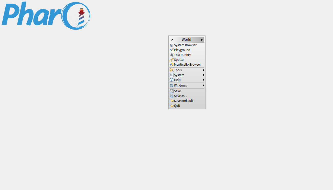
Clicking anywhere on the background of the Pharo window will display the World Menu. World Menu contains many of the Pharo tools, utilities and settings.
You will see a list of several core tools in Pharo, including the class browser and the workspace.
5. Install Kendrick
From the the World Menu, select the "Tools" and after that the Configuration Browser. Find in the Configuration Browser, the Kendrick configuration and select it. Click on "Install Stable version". You need to be connected to the Internet, in order to download the Kendrick package.
6. Finding out the Examples package integrated in Kendrick
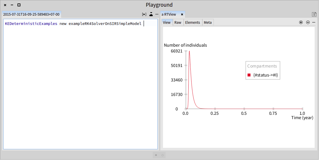
From the World menu, select the "System Browser". Type "Kendrick" in the searching textbox to find the Kendrick packages then expanding "Kendrick". All the integrated examples of Kendrick could be found in the "Examples" package. To run an example, from the World menu, select Workspace. In the Playground form, type a script to create an example and run it. For example:
KEDeterministicExamples new exampleRK4SolverOnSIRSimpleModel
KEDeterministicExamples: class name.
exampleRK4SolverOnSIRSimpleModel: method name.
Then click on the play button to run the script. The result will be represented in the next view (Figure 6.1)
7. Launching models with simulation tools of Kendrick
An epidemiological model can be interpreted to run a deterministic, stochastic or agent-based simulation. The simulations are written once but for all the Kendrick models.
Once the model is specified, create new instance of KESimulator and determine the parameters of simulation such as: algorithm, starting time, ending time and the step. For example:
simulator := KESimulator new: #RungeKutta from: 0.0 to: 1.0 step: 0.001.
simulator executeOn: model.
For this moment, the platform supported the algorithms: ODE Solvers (RungeKutta, Euler, etc.), Gillespie's direct, Explicit Tau Leap and Individual-based simulation. The scripts following allows to create these simulations:
simulator := KESimulator new: #Gillespie from: 0.0 to: 1.0 step: 0.001.
simulator executeOn: model.
simulator := KESimulator new: #TauLeap from: 0.0 to: 1.0 step: 0.001.
simulator executeOn: model.
simulator := KESimulator new: #IBM from: 0.0 to: 1.0 step: 0.001.
simulator executeOn: model.
In Kendrick platform, the simulation results are stored as time series.
simulator allTimeSeries
This script will return an array of all time series. To obtain the time series of a compartment, just indicate the name of this compartment as parameter of the function "timeSeriesAt".
simulator timeSeriesAt: '{#status: #I}'
These scripts below allow to apply an additional function on the time series.
(simulator timeSeriesAt: '{#status: #I}') sqrt
(simulator timeSeriesAt: '{#status: #I}') log
The time series then are passed as data of the diagram builder to view the simulation results:
diag := (KEDiagramBuilder new) data: simulator allTimeSeries.
diag open
Other configurations of diagram:
diag xLabel: 'Time (years)'.
diag yLabel: 'Infectious'.
diag legendTitle: 'Vaccination rate'
By default, xLabel: Time (days), yLabel: Number of individuals, legendTitle: Compartments.