Introduction to Simple Epidemic Model
The targeted model of the Kendrick language is compartmental model such as the SIR, SEIR model ... in which the individuals are first considered as Susceptible to pathogen (status S), then can be infected, assumed Infectious (status I) that can spread the infection and Recovery (status R) who are immunised and cannot become infected again. The transition of status between compartments is represented mathematically as derivatives of compartment size with respect to time.
At the moment, Kendrick supports for the mathematical models of epidemiology based on ordinary differential equations (ODEs). The system of ODEs followed represents the SIR classic model of epidemiology:
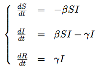
These models are specified using the Kendrick language and modeled using the simulation module integrated into the platform. The simulator takes the Kendrick model (the epidemiological model written in Kendrick language) and performs a simulation algorithm and give out the result showing the spatial and temporal evolution dynamics of each compartment. This visualization is done by using Roassal.
The simulation module supports three modeling formalisms: deterministic, stochastic and individual-based (also called agent-based). The modelers can switch between the simulation modes by indicating the algorithm used. At the moment, we use the RK4 method for deterministically resolving ODEs. The stochastic simulation converts the ODEs of the model to events and using Gillespie's algorithms to generate stochastic model. The individual-based simulator allows to reach the model at more detailed level.
1. Simple SIR (without births and deaths)
Program 2.1 is a simple SIR model. These are the equations and the code of the model:
1.1. Equations
1.2. Pharo code
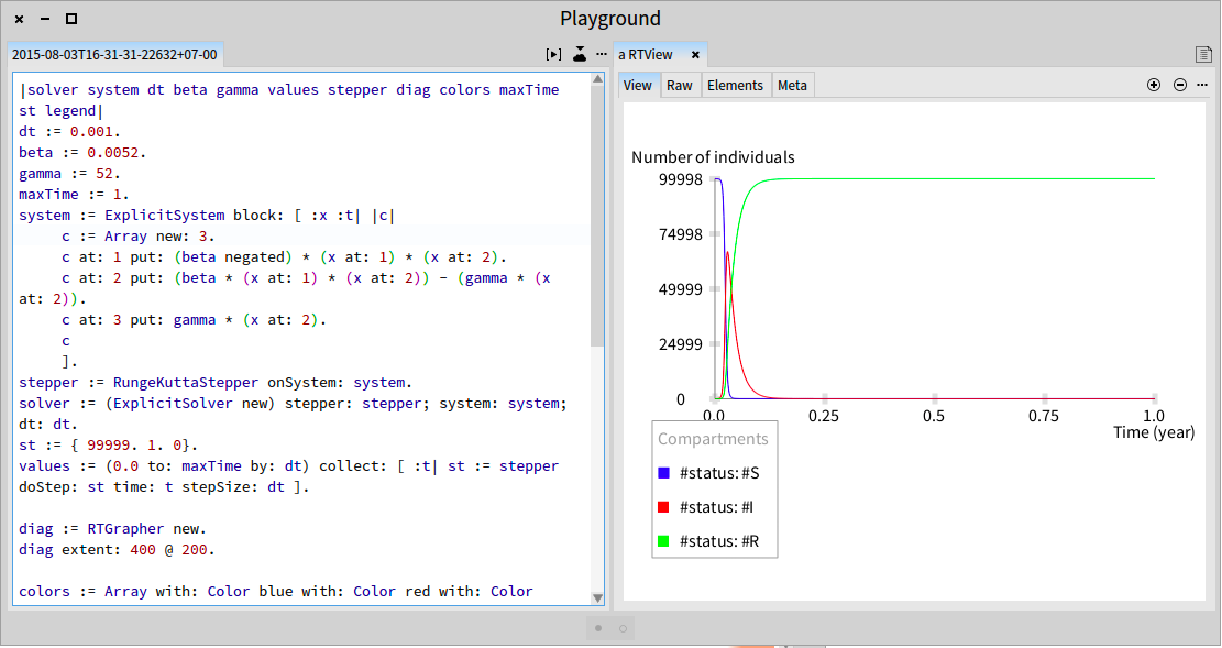
Here, we just demonstrate the code written in Smalltalk language to resolve the system of equations and view the results.
|solver system dt beta gamma values stepper diag colors maxTime st legend|
dt := 0.001.
beta := 0.0052.
gamma := 52.
maxTime := 1.
system := ExplicitSystem block: [ :x :t| |c|
     c := Array new: 3.
     c at: 1 put: (beta negated) * (x at: 1) * (x at: 2).
     c at: 2 put: (beta * (x at: 1) * (x at: 2)) - (gamma * (x at: 2)).
     c at: 3 put: gamma * (x at: 2).
     c
     ].
stepper := RungeKuttaStepper onSystem: system.
solver := (ExplicitSolver new) stepper: stepper; system: system; dt: dt.
st := { 99999. 1. 0}.
values := (0.0 to: maxTime by: dt) collect: [ :t| st := stepper doStep: st time: t stepSize: dt ].

diag := RTGrapher new.
diag extent: 400 @ 200.

colors := Array with: Color blue with: Color red with: Color green.
1 to: 3 do: [ :i|
    |ds|
    ds := RTDataSet new.
    ds points: (1.0 to: ((maxTime/dt)+1) by: 1).
    ds y: [ :x| (values at: x) at: i ].
    ds x: [ :t| (t - 1)*dt].
    ds noDot.
    ds connectColor: (colors at: i).
    diag add: ds ].
diag axisX title: 'Time (year)'.
diag axisY title: 'Number of individuals'.
diag axisY noDecimal.
legend := RTLegendBuilder new.
legend view: diag view.
legend addText: 'Compartments'.
legend addColor: (colors at: 1) text: '#status: #S'.
legend addColor: (colors at: 2) text: '#status: #I'.
legend addColor: (colors at: 3) text: '#status: #R'.
legend build.
diag build.
diag view @ RTZoomableView.
^ diag view
Executing this script we obtain the results of the system of equations as in Figure 1.1
1.3. Kendrick code
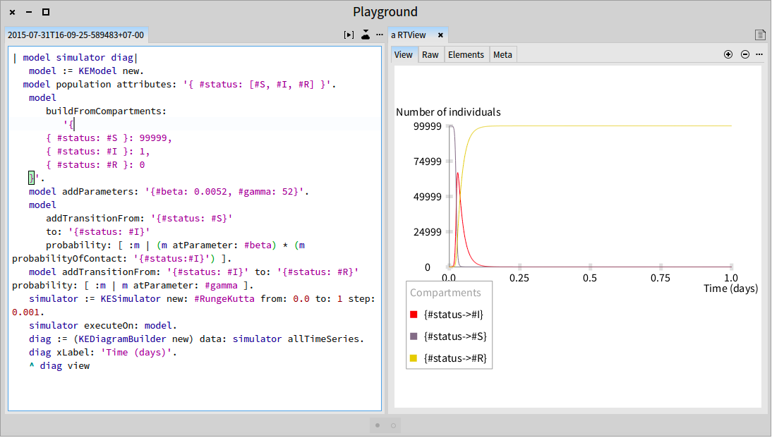
We use now the Kendrick DSL to express the SIR model. We start to create an instance of KEModel and then enumerate the compartment names with their initial value. In this model, we have 3 compartments S, I and R. The population has one attribute status. There is at least one infected in order to start the process. Two transitions are added to the model, one from S to I and another one from I to R. The parameters of the model .
| model |
    model := KEModel new.
  model population attributes: '{ #status: [#S, #I, #R] }'.
    model
        buildFromCompartments:
            '{
        { #status: #S }: 99999,
        { #status: #I }: 1,
        { #status: #R }: 0
    }'.
    model addParameters: '{#beta: 0.0052, #gamma: 52}'.
    model
        addTransitionFrom: '{#status: #S}'
        to: '{#status: #I}'
        probability: [ :m | (m atParameter: #beta) * (m probabilityOfContact: '{#status:#I}') ].
    model addTransitionFrom: '{#status: #I}' to: '{#status: #R}' probability: [ :m | m atParameter: #gamma ].
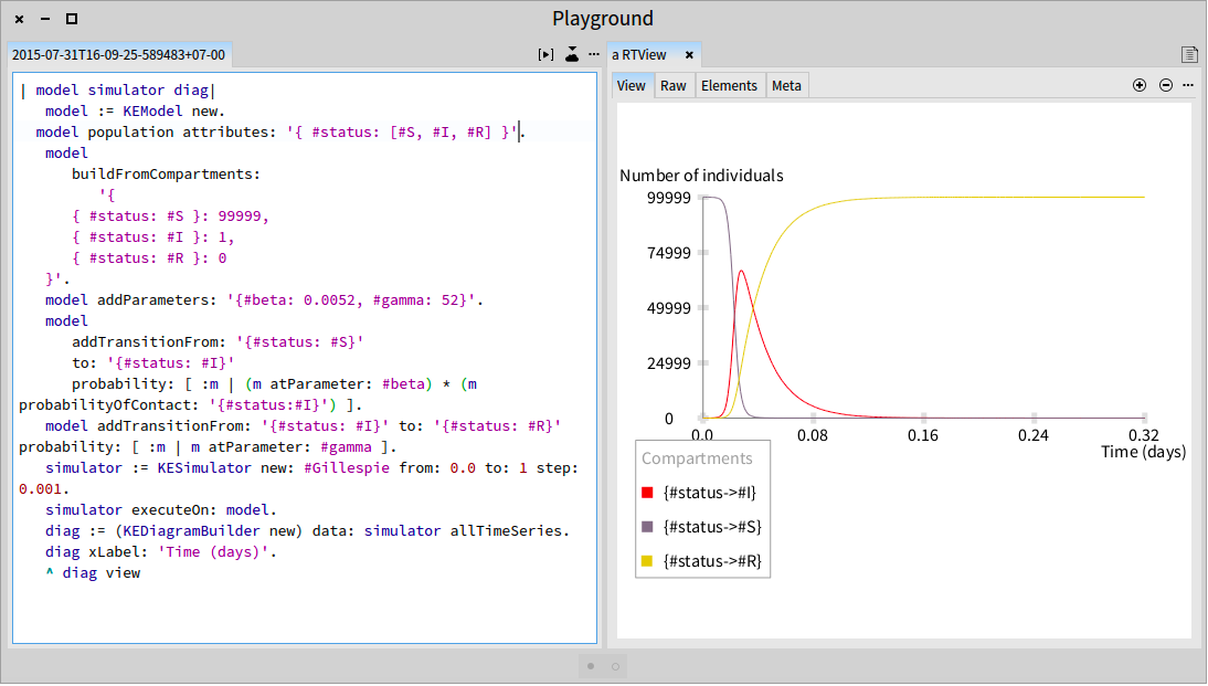
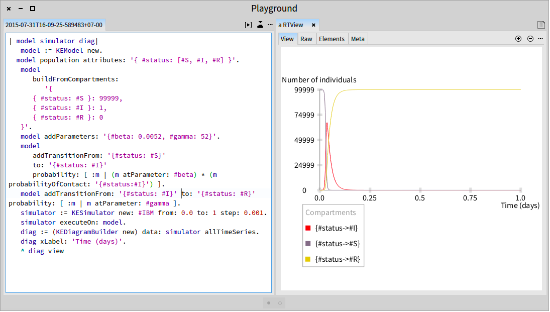
Paste this script in the Workspace tool, define the simulations on this model, we obtain the results as in Figure 1.2. We can find that, the two scripts returns identical results. As a DSL for epidemiology, using Kendrick is more simple. Change the algorithm of simulation from RungeKutta to Gillespie and IBM to investigate two other formalisms (stochastic and agent-based). The results of these simulation are shown in Figure 1.3 and Figure 1.4.
2. SIR model with births and deaths
2.1. Equations
2.2. Pharo code
|solver system dt beta gamma N values stepper diag mu colors maxTime st legend|
dt := 0.1.
mu := 5e-4.
beta := 1/5000.
gamma := 1/10.0.
N := 5000.
maxTime := 146.
system := ExplicitSystem block: [ :x :t| |c|
     c := Array new: 3.
     c at: 1 put: (mu*N) - (beta  * (x at: 1) * (x at: 2)) - (mu * (x at:1)).
     c at: 2 put: (beta * (x at: 1) * (x at: 2)) - (gamma * (x at: 2)) - (mu * (x at:2)).
     c at: 3 put: (gamma * (x at: 2)) - (mu * (x at: 3)).
     c
     ].

stepper := RungeKuttaStepper onSystem: system.
solver := (ExplicitSolver new) stepper: stepper; system: system; dt: dt.
st := #(4975 25 0).
values := (0.0 to: maxTime by: dt) collect: [ :t| st := stepper doStep: st
                                                          time: t stepSize: dt ].
diag := RTGrapher new.
diag extent: 400 @ 200.

colors := Array with: Color blue with: Color red with: Color green.
1 to: 3 do: [ :i|
    |ds|
    ds := RTDataSet new.
    ds points: (1.0 to: ((maxTime/dt)+1) by: 1).
    ds y: [ :x| (values at: x) at: i ].
    ds x: [ :t| (t - 1)*dt].
    ds noDot.
    ds connectColor: (colors at: i).
    diag add: ds ].
diag axisX title: 'Time (days)'.
diag axisY title: 'Number of individuals'.
diag axisY noDecimal.
legend := RTLegendBuilder new.
legend view: diag view.
legend addText: 'Compartments'.
legend addColor: (colors at: 1) text: '#status: #S'.
legend addColor: (colors at: 2) text: '#status: #I'.
legend addColor: (colors at: 3) text: '#status: #R'.
legend build.
diag build.
diag view @ RTZoomableView.
^ diag view
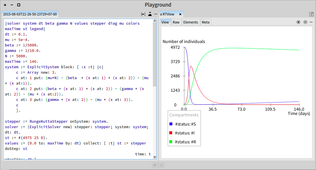
Running this script will give the results as can be seen in Figure 2.1
2.3. Kendrick code
Comparing to the previous model, in this model, it should add four other transitions. The first one represents the births of susceptible. The three others represent the deaths of each compartment. We use the ODE syntax to specify this model.
| model |
    model := KEModel new.
    model population attributes: '{#status: [#S, #I, #R]}'.
  model
        buildFromCompartments:
            '{
        { #status: #S }: 4975,
        { #status: #I }: 25,
        { #status: #R }: 0
    }'.
    model addParameter: #beta value: 1 / 5000.
    model addParameter: #gamma value: 1 / 10.0.
    model addParameter: #mu value: 5e-4.
    model addParameter: #N value: #sizeOfPopulation.
    model addEquation: 'S:t=mu*N-beta*S*I-mu*S' parseAsAnEquation.
    model addEquation: 'I:t=beta*S*I-gamma*I-mu*I' parseAsAnEquation.
    model addEquation: 'R:t=gamma*I-mu*R' parseAsAnEquation.
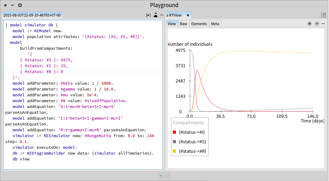
Using deterministic simulation on this model we obtain the result as can be seen in Figure 2.2
3. SEIR model with births and deaths
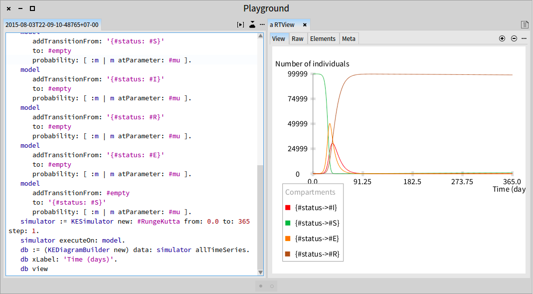
We introduce here a SEIR model. The E status means that a susceptible becomes infected but not yet infectious.
3.1. Equations
3.2. Kendrick code
Here, we use the parameters of measles model. The time unit is day.
| model |
    model := KEModel new.
    model population attributes: '{#status: [#S, #E, #I, #R]}'.
    model
        buildFromCompartments:
            '{
        {#status: #S}: 99999,
        {#status: #I}: 1,
        {#status: #E}: 0,
        {#status: #R}: 0
    }'.
    model addParameters: '{
        #beta: 0.0000214,
        #gamma: 0.143,
        #mu: 0.0000351,
        #sigma: 0.125,
        #N: #sizeOfPopulation}'.
    model
        addTransitionFrom: '{#status: #S}'
        to: '{#status: #E}'
        probability: [ :m | (m atParameter: #beta) * (m probabilityOfContact: '{#status:#I}') ].
    model
        addTransitionFrom: '{#status: #E}'
        to: '{#status: #I}'
        probability: [ :m | m atParameter: #sigma ].
    model
        addTransitionFrom: '{#status: #I}'
        to: '{#status: #R}'
        probability: [ :m | m atParameter: #gamma ].
    model
        addTransitionFrom: '{#status: #S}'
        to: #empty
        probability: [ :m | m atParameter: #mu ].
    model
        addTransitionFrom: '{#status: #I}'
        to: #empty
        probability: [ :m | m atParameter: #mu ].
    model
        addTransitionFrom: '{#status: #R}'
        to: #empty
        probability: [ :m | m atParameter: #mu ].
    model
        addTransitionFrom: '{#status: #E}'
        to: #empty
        probability: [ :m | m atParameter: #mu ].
    model
        addTransitionFrom: #empty
        to: '{#status: #S}'
        probability: [ :m | m atParameter: #mu ].
4. SEIR model with vaccination at births
4.1. Equations
4.2. Kendrick code
| model |
    model := KEModel new.
    model population attributes: '{#status: [#S, #E, #I, #R]}'.
    model
        buildFromCompartments:
            '{
        {#status: #S}: 99999,
        {#status: #I}: 1,
        {#status: #E}: 0,
        {#status: #R}: 0
    }'.
    model addParameters: '{
        #beta: 0.00782,
        #gamma: 52.14,
        #mu: 0.0128,
        #sigma: 45.625,
        #N: #sizeOfPopulation,
        #p: 0.7}'.
    model
        addTransitionFrom: '{#status: #S}'
        to: '{#status: #E}'
        probability: [ :m | (m atParameter: #beta) * (m probabilityOfContact: '{#status:#I}') ].
    model
        addTransitionFrom: '{#status: #E}'
        to: '{#status: #I}'
        probability: [ :m | m atParameter: #sigma ].
    model
        addTransitionFrom: '{#status: #I}'
        to: '{#status: #R}'
        probability: [ :m | m atParameter: #gamma ].
    model
        addTransitionFrom: '{#status: #S}'
        to: #empty
        probability: [ :m | m atParameter: #mu ].
    model
        addTransitionFrom: '{#status: #I}'
        to: #empty
        probability: [ :m | m atParameter: #mu ].
    model
        addTransitionFrom: '{#status: #R}'
        to: #empty
        probability: [ :m | m atParameter: #mu ].
    model
        addTransitionFrom: '{#status: #E}'
        to: #empty
        probability: [ :m | m atParameter: #mu ].
    model
        addTransitionFrom: #empty
        to: '{#status: #S}'
        probability: [ :m | (m atParameter: #mu) * (1 - (m atParameter: #p)) ].
    model
        addTransitionFrom: #empty
        to: '{#status: #R}'
        probability: [ :m | (m atParameter: #mu) * (m atParameter: #p) ].
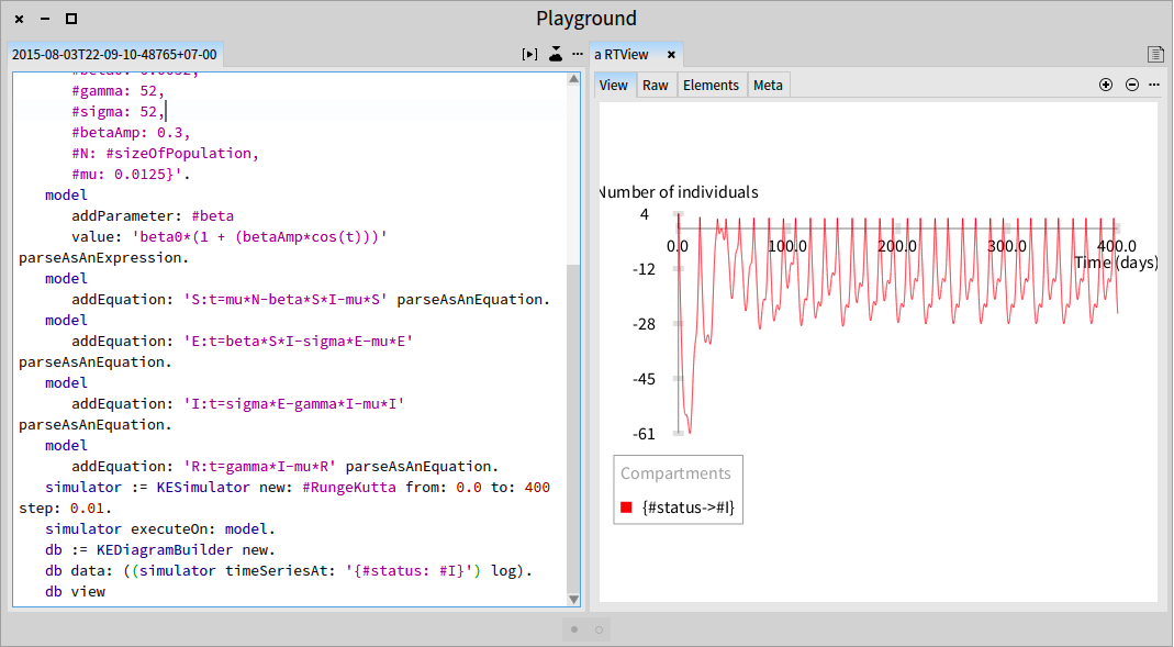
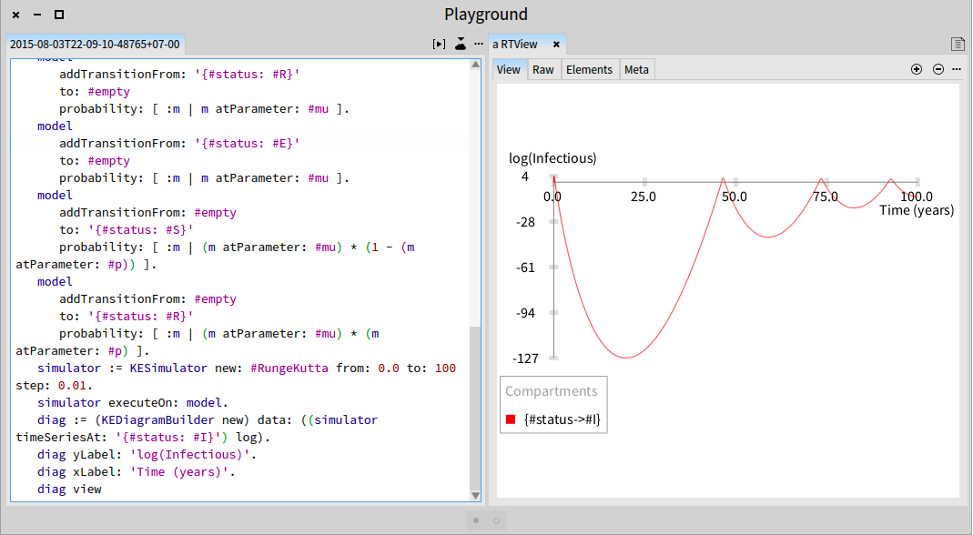
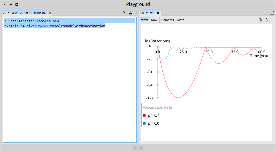
Here we take the vaccination rate . In order to study the vaccination effect, we change the value of and compare the two case as in Figure 4.1. After running a simulation on the first model (with p = 0.7), we reset the model with the command:
model resetCompartments
The script to show this comparison can be found in the Examples package of Kendrick. The parameters of Kendrick model is not only a constant but also a temporal function as in this model. The Y-axis is loged for readibilty.
5. SEIR model with seasonal forcing
5.1. Equations
5.2. Kendrick code
| model |
    model := KEModel new.
    model population attributes: '{ #status: [#S, #E, #I, #R] }'.
    model
        buildFromCompartments:
            '{
        { #status: #S }: 99999,
        { #status: #E }: 0,
        { #status: #I }: 1,
        { #status: #R }: 0
    }'.
    model addParameters: '{
        #beta0: 0.0052,
        #gamma: 52,
        #sigma: 52,
        #betaAmp: 0.3,
        #N: #sizeOfPopulation,
        #mu: 0.0125}'.
    model
        addParameter: #beta
        value: 'beta0*(1 + (betaAmp*cos(t)))' parseAsAnExpression.
    model
        addEquation: 'S:t=mu*N-beta*S*I-mu*S' parseAsAnEquation.
    model
        addEquation: 'E:t=beta*S*I-sigma*E-mu*E' parseAsAnEquation.
    model
        addEquation: 'I:t=sigma*E-gamma*I-mu*I' parseAsAnEquation.
    model
        addEquation: 'R:t=gamma*I-mu*R' parseAsAnEquation.